The Theory of Coupled Oscillators

It is a common joke that theoretical physics is just largely the study of a single system – the harmonic oscillator. It is true that this system is primarily the most complicated system that can be fully solved analytically, but it is also true that it is so simple that nearly any high school student is familiar with its general form. A harmonic oscillator stems from a restoring force, or a force that is negatively proportional to some measurable quantity:

$F=-kx$

where $k$ is the proportional factor and $x$ is the measurable quantity. The equation of motion corresponding to this force can be found by considering Newton’s Second Law $F=ma$ :

$m\frac{d^2x}{dt^2}=-kx$

By rearranging this equation and defining $\omega^2=k/m$ , we can see that we have an eigenequation for the second order differential operator $\frac{d^2}{dt^2}$ with eigenfunction $x$ and eigenvalue $-\omega^2$ :

$\frac{d^2}{dt^2}x=-\omega^2 x$

Our goal then is to find the function $x(t)$ that has the property that when it is acted upon by the operator $\frac{d^2}{dt^2}$ , it results in the same function $x(t)$ multiplied by a constant $-\omega^2$ . When it comes to differentiating functions and returning the same function, the exponential function $e^t$ immediately comes to mind. Let’s try $x(t)=e^{\omega t}$ for our eigenfunction then. Differentiating twice, we see that $\ddot{x}(t) = \omega^2 x(t)$ . Unfortunately, we are missing a minus sign. What other function could we try? Interestingly, we find that we can resolve this issue by introducing the imaginary number $i$ . If we try $x(t)=e^{i\omega t}$ for our eigenfunction, we find that $\dot{x}(t)=i\omega e^{\i\omega t}$ and $\ddot{x}(t) = i^2 \omega^2 e^{i\omega t}=-\omega^2 e^{i\omega t}$ . 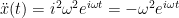Thus we can conclude that $x(t)=e^{i\omega t}$ is an eigenfunction of our equation above. Since our operator is a second-order and linear, we know that the general solution must be the sum of two linearly independent solutions. We already found one solution, $e^{i\omega t}$ , and it is easy to show that another solution $e^{-i\omega t}$ is both also a solution to the eigenequation and is linearly independent of the first solution (since it cannot be obtained by multiplying the first solution by a constant). Thus our general solution for the harmonic oscillator eigenfunction is:

$x(t)=Ae^{i\omega t} + Be^{-i\omega t}$

We have included the constants $A$ and $B$ due to the linearity of the operator (i.e. if $x(t)$ is a solution then $Cx(t)$ must also be a solution where $C$ is an arbitrary constant). In our case, the two constants will be determined by the initial conditions of the system (of which there must be two to completely define the system). Now that we have a solution in hand, what does it mean? What does the harmonic oscillator actually look like? Using Euler’s formula, we can rewrite our general solution as:

$x(t)=A(\cos(\omega t)+i\sin(\omega t))+B(\cos(\omega t)-i\sin(\omega t))$

Taking the real part of this, we get:

$\text{Re}(x(t)) = A\cos(\omega t) + B\cos(\omega t)$

So we can see that the harmonic oscillator behaves like a sine wave. Simple enough – anyone who has ever observed a spring can tell you that this is indeed its behavior. However, if we want to model real systems, sometimes a single spring isn’t enough. For example, let’s consider the case of the structure of a protein. A protein is a polymer made up of subunits called amino acids. Each amino acid sits in a linear chain and is connected to its neighbors by a chemical bond. We can represent this chemical bond as a spring, which means that the protein as a whole is just a collection of springs that are coupled to each other. In other words, each spring no longer oscillates independently – its motion depends also on the springs it is coupled to, and vice versa. How do we describe the motion of the harmonic oscillators in this case?

Let’s try to look at a simpler system first and see how the tools of mathematics allow us to solve the system. Let’s consider the simplest case of coupled oscillators – two masses and three springs. Consider the system shown in the figure below, where we have two masses of mass $m_1$ and $m_2$ connected by a total of three springs with spring constants $k_1$ , $k_2$ , and $k_3$ . The spring with $k_1$ constant connects the mass $m_1$ to a wall, the spring with $k_2$ constant connects masses $m_1$ and $m_2$ , and the spring with $k_3$ constant connects mass $m_2$ to another wall. The walls do not move.

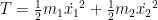
Let us assume that when the springs are at their equilibrium position (i.e. when they are unstretched or uncompressed and there is no restoring force present), they are all of equal length and all the masses are at rest. We can describe any perturbation of the masses from this equilibrium position using the parameters $x_1$ and $x_2$ . These are the only two variables we will need to determine the system, as there are two degrees of freedom present (the positions of the two masses). Note that it is not three degrees of freedom since if we know the positions of the two masses, we can also deduce the lengths of each of the three springs. Using the Lagrangian approach described in a previous post, our first step is to write the kinetic and potential energies of this system in terms of our two parameters $x_1$ and $x_2$ . The kinetic energy terms are simply the kinetic energy $\frac{1}{2}mv^2$ given by the motion of the two masses:

$T=\frac{1}{2}m_1\dot{x_1}^2+\frac{1}{2}m_2\dot{x_2}^2$

The potential energy terms are a little trickier. The energy of a spring can be obtained through the general force-energy relationship:

$V=-\int F(x)\,dx = -\int kx\,dx = \frac{1}{2}kx^2$

So all we need to know is the displacement of the spring and we can write the energy. From looking at the diagram, it is clear that the displacement for spring 1 is just $x_1$ and the displacement for spring 3 is just $x_2$ . What about the displacement for spring 2? Let us imagine moving both of the masses some distance $x_1$ and $x_2$ , respectively. Then spring 2 will have been shifted by a displacement $x_2-x_1$ , as long as we assume that “right” is the positive direction. Now that we have our displacements, we can write the total potential energy of the system:

$V=\frac{1}{2}k_1 x_1^2 + \frac{1}{2}k_3 x_2^2 + \frac{1}{2}k_2(x_2-x_1)^2$

Now we can write the Lagrangian:

$L=T-V=\frac{1}{2}m_1\dot{x_1}^2+\frac{1}{2}m_2\dot{x_2}^2 - \frac{1}{2}k_1 x_1^2 - \frac{1}{2}k_3 x_2^2 - \frac{1}{2}k_2 (x_2-x_1)^2$

Since we have two degrees of freedom here, we will write two Euler-Lagrange equations, each one corresponding to either the parameter $x_1$ or $x_2$ . The first one is shown below:

$\frac{\partial L}{\partial x_1}=\frac{d}{dt}\left(\frac{\partial L}{\partial \dot{x}_1}\right) \\[10pt] \Rightarrow -k_1 x_1 + k_2 \left(x_2-x_1\right)=\frac{d}{dt}\left(m_1 \dot{x}_1\right) \\[10pt] \phantom{\Rightarrow} -\left(k_1+k_2\right) x_1+k_2 x_2=m_1\ddot{x}_1$

The second one is:

$\frac{\partial L}{\partial x_2}=\frac{d}{dt}\left(\frac{\partial L}{\partial \dot{x}_2}\right) \\[10pt] \Rightarrow -k_3 x_2 - k_2\left(x_2-x_1\right)=\frac{d}{dt}\left(m_2\dot{x}_2\right) \\[10pt] \phantom{\Rightarrow} k_2 x_1 - \left(k_3+k_2\right) x_2 = m_2\ddot{x}_2$

So now we have obtained our two coupled equations of motion of the system from the Euler-Lagrange equations:

$m_1\ddot{x}_1=-\left(k_1+k_2\right) x_1+k_2 x_2 \\[10pt] m_2\ddot{x}_2=k_2 x_1 - \left(k_2+k_3\right)x_2$

Note that we can write these equations in matrix form:

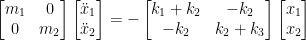
$\begin{bmatrix} m_1 & 0 \\ 0 & m_2 \end{bmatrix} \begin{bmatrix} \ddot{x}_1 \\ \ddot{x}_2 \end{bmatrix} = -\begin{bmatrix} k_1+k_2 & -k_2 \\ -k_2 & k_2+k_3 \end{bmatrix} \begin{bmatrix} x_1 \\ x_2 \end{bmatrix}$

or simply:

$\mathbf{M \ddot{x}}=-\mathbf{Kx}$

where we call $\mathbf{M}$ the mass matrix and $\mathbf{K}$ the spring constant matrix. By multiplying out the matrices you can convince yourself that this does accurately represent our two coupled equations of motion. Note that our matrix equation $\mathbf{M\ddot{x}}=-\mathbf{Kx}$ is also just a generalization of the one-dimensional spring force equation $m\ddot{x}=-kx$ .

Now, our goal is to solve for the vector $\mathbf{x}$ as a function of time, as this will fully describe the motion of the system. To do this, since we know our differential operator is linear from earlier, we just need to find two linearly independent solutions for $\mathbf{x}(t)$ . Then a linear combination of those two solutions will give us our general solution. The reason we choose two solutions specifically is because we have already determined that our system only has two degrees of freedom. Two linearly independent solutions, then, will be able to span the whole space of the system.

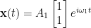
How do we go about finding these two linearly independent solutions? The first step to solving any differential equation is guessing – let us guess a solution, plug it into our equations of motion, and see if it works! Luckily for us, we already have a good starting point – we have already determined that a solution $Ae^{i\omega t}$ is a solution for the single harmonic oscillator. What if we tried this solution for our coupled oscillator system? In other words, let’s try the solution:

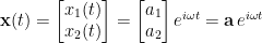
$\mathbf{x}(t) = \begin{bmatrix} x_1(t) \\ x_2(t) \end{bmatrix} = \begin{bmatrix} a_1 \\ a_2 \end{bmatrix} e^{i\omega t} = \mathbf{a}\, e^{i\omega t}$

Note that in our “made-up” solution, we have that both masses are oscillating at the same frequency $\omega$ , albeit at different amplitudes – mass 1 is oscillating with an amplitude $a_1$ and mass 2 is oscillating with an amplitude $a_2$ . Cases like these, where all the parts in a system are oscillating at the same frequency, are called normal modes. The next step is to plug our solution into our differential equation. Computing the derivatives of our solution, we have:

$\mathbf{x}(t) = \mathbf{a}\,e^{i\omega t} \\[10pt] \mathbf{\dot{x}}(t) = i\omega\,\mathbf{a}\,e^{i\omega t} \\[10pt] \mathbf{\ddot{x}}(t)=i^2\omega^2\mathbf{a}\,e^{i\omega t} = -\omega^2\mathbf{a}\,e^{i\omega t}$

Plugging these into our differential equation $\mathbf{M \ddot{x}}=-\mathbf{Kx}$ , we get:

$-\omega^2\mathbf{Ma}\,e^{i\omega t}=-\mathbf{Ka}\,e^{i\omega t}$

Cancelling out the $e^{i\omega t}$ ‘s on both sides, we get:

$-\omega^2\mathbf{Ma}=-\mathbf{Ka} \\[10pt] \Rightarrow \omega^2\mathbf{Ma}+\mathbf{Ka} = 0 \\[10pt] \phantom{\Rightarrow} \left(\mathbf{K}-\omega^2\mathbf{M}\right)\mathbf{a}=0$

Note that what we have here is an eigenequation, similar to what we had before for the single oscillator case. In this case, our operator is the matrix $\left(\mathbf{K}-\omega^2\mathbf{M}\right)$ and it is acting on the vector $\mathbf{a}$ to return a value of 0. Our goal is to solve for the eigenvalue $\omega$ that makes this relation true, which we can then use to find our eigenvector $\mathbf{a}$ . First, we see that $\mathbf{a}=0$ is obviously one possible solution. In this solution, neither of the masses are moving – thus this is the equilibrium solution. Clearly this solution, while certainly a valid one, is of little interest to us. So let’s take a leap of faith and postulate that there must exist nontrivial solutions. Representing our matrix $\left(\mathbf{K}-\omega^2\mathbf{M}\right)$ as simply $\mathbf{A}$ , we shall state that the equation $\mathbf{Ax}=0$ does not only have the trivial solution $\mathbf{x}=0$ . If this is true, then it tells us that our matrix $\mathbf{A}$ is not an invertible matrix. A property of an invertible matrix $\mathbf{A}$ is that $\text{det}(\mathbf{A})\neq 0$ . Since we know our matrix $\mathbf{A}$ is not invertible, it must be true that $\text{det}(\mathbf{A})=0$ . In short, in order to find our eigenvalue $\omega$ , we just have to solve the equation $\text{det}(\mathbf{A})=0$ , i.e. $\text{det}\left(\mathbf{K}-\omega^2\mathbf{M}\right)=0$ . Proceeding, we have that:

$\mathbf{K}-\omega^2\mathbf{M}=\begin{bmatrix}k_1+k_2 & -k_2 \\ -k_2 & k_2+k_3\end{bmatrix}-\begin{bmatrix}\omega^2 m_1 & 0 \\ 0 & \omega^2 m_2\end{bmatrix} \\[10pt] \phantom{\mathbf{K}-\omega^2\mathbf{M}} = \begin{bmatrix} k_1+k_2-\omega^2 m_1 & -k_2 \\ -k_2 & k_2+k_3-\omega^2 m_2\end{bmatrix}$

Finding the determinant of a 2×2 matrix is easy, so we compute:

$\text{det}\left(\mathbf{K}-\omega^2\mathbf{M}\right)=\left(k_1+k_2-m_1\omega^2\right)\left(k_2+k_3-m_2\omega^2\right)-(-k_2)(-k_2)=0$

Trying to solve this with a symbolic solver such as Wolfram Alpha gives the following result:

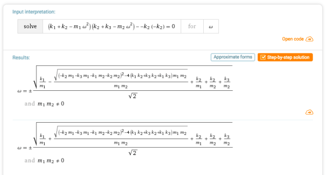
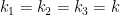Clearly a solution does exist, but it is so unwieldy that we cannot really do much more with it. Let’s try a simpler case, then. Let’s reframe our problem so that all the masses and all the springs are identical, i.e. $m_1=m_2=m$ and $k_1=k_2=k_3=k$ . Then our spring constant and mass matrices simplify to:

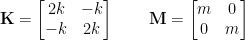
$\mathbf{K}=\begin{bmatrix}2k & -k \\ -k & 2k\end{bmatrix} \hspace{25pt} \mathbf{M}=\begin{bmatrix}m&0\\0&m\end{bmatrix}$

$\mathbf{K}-\omega^2\mathbf{M}=\begin{bmatrix}2k & -k \\ -k & 2k \end{bmatrix} - \begin{bmatrix} \omega^2 m & 0 \\ 0 & \omega^2 m \end{bmatrix} = \begin{bmatrix} 2k-\omega^2 m & -k \\ -k & 2k-\omega^2 m\end{bmatrix}$

And we can solve $\text{det}\left(\mathbf{K}-\omega^2\mathbf{M}\right)=0$ :

$\text{det}\left(\mathbf{K}-\omega^2\mathbf{M}\right)=\left(2k-m\omega^2\right)^2-k^2 = 0 \\[10pt] \Rightarrow 3k^2-4km\omega^2+m^2\omega^4=0 \\[10pt] \phantom{\Rightarrow} \left(2k-m\omega^2\right)\left(k-m\omega^2\right)=0 \\[10pt] \Rightarrow \omega=\sqrt{\frac{3k}{m}}, \sqrt{\frac{k}{m}}$

We see that we have two solutions for $\omega$ , which suggests that we have two normal mode frequencies. Note that we have excluded the negative solutions of $\omega$ , since frequencies are invariant to sign change. Now that we have the eigenvalues $\omega$ in hand, we can solve for the corresponding eigenvectors $\mathbf{a}$ by plugging the eigenvalues $\omega$ back into the equation 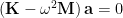$\left(\mathbf{K}-\omega^2\mathbf{M}\right)\mathbf{a}=0$ . For the first eigenvalue $\omega_1=\sqrt{\frac{k}{m}}$ , we have:

$\omega_1^2=\frac{k}{m} \Rightarrow \left(\begin{bmatrix}2k & -k \\ -k & 2k\end{bmatrix}-\begin{bmatrix}m\frac{k}{m} & 0 \\ 0 & m \frac{k}{m}\end{bmatrix}\right)\mathbf{a}=0 \\[10pt] \phantom{\omega_1^2=\frac{k}{m} \Rightarrow} \begin{bmatrix}k & -k \\ -k & k\end{bmatrix}\mathbf{a} =0 \\[10pt] \phantom{\omega_1^2=\frac{k}{m} \Rightarrow}\begin{bmatrix}1 & -1 \\ -1 & 1\end{bmatrix}\begin{bmatrix}a_1 \\ a_2 \end{bmatrix}=0$

We can solve this matrix problem by row-reducing the following equivalent matrix:

$\begin{pmatrix}-1 & -1 & 0 \\ -1 & 1 & 0\end{pmatrix} \\[10pt] \begin{pmatrix} 1 & -1 & 0 \\ 0 & 0 & 0 \end{pmatrix} \\[10pt] \Rightarrow a_1 - a_2 = 0 \\[10pt] \phantom{\Rightarrow} a_1 = a_2$

So we have that $a_1=a_2$ for our first normal mode. In other words, in this mode our masses are oscillating at the same frequencies and the same amplitudes. Since we only have one equation for two variables, our variables are undetermined and can be set to anything, so let’s just set $a_1=a_2=A_1$ . So our first normal mode solution is:

$\mathbf{x}(t)=A_1\begin{bmatrix}1 \\ 1\end{bmatrix}e^{i\omega_1 t}$

For the second eigenvalue $\omega_2=\sqrt{\frac{3k}{m}}$ , we have:

$\omega_2^2=\frac{3k}{m} \Rightarrow \left(\begin{bmatrix}2k & -k \\ -k & 2k\end{bmatrix}-\begin{bmatrix}m\frac{3k}{m} & 0 \\ 0 & m \frac{3k}{m}\end{bmatrix}\right)\mathbf{a}=0 \\[10pt] \phantom{\omega_1^2=\frac{k}{m} \Rightarrow} \begin{bmatrix}-k & -k \\ -k & -k\end{bmatrix}\mathbf{a} =0 \\[10pt] \phantom{\omega_1^2=\frac{k}{m} \Rightarrow}\begin{bmatrix}-1 & -1 \\ -1 & -1\end{bmatrix}\begin{bmatrix}a_1 \\ a_2 \end{bmatrix}=0 \\[10pt] \phantom{\omega_1^2=\frac{k}{m} \Rightarrow}\begin{pmatrix}-1 & -1 & 0 \\ -1 & -1 & 0\end{pmatrix} \\[10pt] \phantom{\omega_1^2=\frac{k}{m} \Rightarrow}\begin{pmatrix} 1 & 1 & 0 \\ 0 & 0 & 0 \end{pmatrix} \\[10pt] \phantom{\omega_1^2=\frac{k}{m}}\Rightarrow a_1 + a_2 = 0 \\[10pt] \phantom{\omega_1^2=\frac{k}{m} \Rightarrow}\phantom{\Rightarrow} a_1 = -a_2$

In the second normal mode, the masses are oscillating at the same frequency but with exactly opposite amplitudes. Like before, the specific amplitude is undetermined, so we can just set 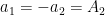$a_1=-a_2=A_2$ . So our second normal mode solution is:

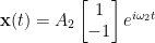
$\mathbf{x}(t)=A_2\begin{bmatrix}1\\-1\end{bmatrix}e^{i\omega_2 t}$

So now we can write our general solution as a linear sum of these two normal modes:

$\mathbf{x}(t) = A_1\begin{bmatrix}1\\1\end{bmatrix}e^{i\omega_1 t}+A_2\begin{bmatrix}1\\-1\end{bmatrix}e^{i\omega_2 t}$

Note that we expect four total constants in this equation to account for the four total initial conditions we need to completely determine the system (the initial positions and velocities of each of the two masses). At a first glance, it appears that we only have two, $A_1$ and $A_2$ . However, our amplitude values can be complex, so we can separate out the imaginary part from the real part:

$A_1=\alpha_1 e^{-i\delta_1} \\[10pt] A_2=\alpha_2 e^{-i\delta_2}$

And we have our final solution:

$\mathbf{x}(t)=\alpha_1\begin{bmatrix}1\\1\end{bmatrix}e^{i\left(\omega_1 t-\delta_1\right)} + \alpha_2\begin{bmatrix}1\\-1\end{bmatrix}e^{i\left(\omega_2 t-\delta_2\right)} \\[10pt] \text{where} \hspace{10pt} \omega_1=\sqrt{\frac{k}{m}}\hspace{10pt}\text{and}\hspace{10pt}\omega_2=\sqrt{\frac{3k}{m}} \\[10pt] \text{and}\hspace{10pt}\alpha_1, \alpha_2, \delta_1, \delta_2\hspace{10pt} \text{are real numbers determined by initial conditions.}$

Note that the appearance of the $\delta$ ‘s allow for there to be a phase difference between the two different frequencies, leading to some very complicated waveforms in the general solution. To plot an example of a solution, we can use the following Matlab code:

t = linspace(0,10,1000);
k = 50;
m = 5;
omega_1 = sqrt(k/m);
omega_2 = sqrt(3*k/m);
alpha_1 = 1;
alpha_2 = 0.7;
delta_1 = 0;
delta_2 = pi/2;
x = alpha_1*[1;1]*exp(i*(omega_1*t-delta_1))+alpha_2*[1;-1]*exp(i*(omega_2*t-delta_2));
x_real = real(x);
plot(t,x_real)
set(gca,'FontSize',18)
xlabel('Time')
ylabel('Position')
legend('Mass 1','Mass 2')

This results in a nice plot of the positions of our two masses as a function of time:

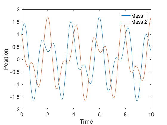
It should be clear now what the general approach to solving coupled-oscillator problems is. In a nutshell:

Write the Lagrangian of the system and use the Euler-Lagrange equations to write the equations of motion.
Write the matrix form of the equations of motion: $\mathbf{M\ddot{x}}=-\mathbf{Kx}$
Find the normal mode frequencies $\omega$ by solving $\text{det}\left(\mathbf{K}-\omega^2\mathbf{M}\right)=0$ .
Plug these normal mode frequencies back into the equation $\left(\mathbf{K}-\omega^2\mathbf{M}\right)\mathbf{a}=0$ to solve for the eigenvectors $\mathbf{a}$ .
Write the general solution as a sum of each normal mode frequency: $\mathbf{x}(t) = \sum_{n}\mathbf{a_n}e^{i\left(\omega_n t-\delta_n\right)}$

Tags: matlab, oscillators, physics, theory

One comment

Haseen · November 30, 2022 - 5:39 am · Reply→

Thank You it is so much explanatory to understand.

LikeLike

Jeremy Kao

The Theory of Coupled Oscillators

One comment

Leave a Reply Cancel reply

Jeremy Kao

The Theory of Coupled Oscillators

Share this:

Like this:

One comment

Leave a Reply Cancel reply