Applied mathematics has always fascinated me because it’s all about solving the most simple problems in the most efficient way. Optimization, for example, is one of the most useful problem people commonly encounter. The premise is simple: Given some number of independent variables that govern some dependent variable, what is the choice of the values for the independent variables that result in the lowest (or highest) possible value for the dependent variable? For example, let’s say you own a shop. As the shop owner, you have the power to vary the number of items you have stocked, the prices of those items, the number of employees you have, etc.  The dependent variable here is the amount of money you earn. So, what is the correct number to place all these variables at to ensure the highest profit? An entire branch of mathematics is dedicated to solving this very type of problem.

Let’s present a toy version of this problem. Suppose you have some scalar function that depends on only one variable, , over some specified finite domain. We would like to ask an optimization question – what value of results in the lowest value for ? The obvious method is a brute-force search – we could simply iterate over all the possible values of , compute the associated value , and select the value of that gives the highest value of . However, such a search is in time complexity for a function of one variable, for a function of two variables, and so on. For most real applications, there can be hundreds or even thousands of independent variables, making a brute-force search completely impractical in most cases, even with modern supercomputing hardware.

So, although a brute-force method is guaranteed to find the global optimum, it is impractical to implement. A gradient descent method is guaranteed to find a local optimum, but has no way of checking if it is actually the global optimum. What we need is something in between – a method that doesn’t search the whole space of the problem but also doesn’t fall into the trap of being stuck in the first local optimum it finds. Simulated annealing is one of the many approximation methods developed to address this problem. The basic principle behind this algorithm is that it will tend to find local optima, but there will always exist some probability that it will sometimes accept a poorer choice, i.e. something not optimal. This is the way that it avoids being trapped in local optima – there will always be a chance that it will jump out and continue searching for a better optimum. The mathematical formulation of this algorithm provides a quantitative way to balance the costs of leaving a local optimum with the benefits of perhaps finding a better optimum. In this post, we will apply the simulated annealing algorithm to our simple case of finding the global minimum of a function of one variable, . First, let’s outline the steps of the algorithm:

1. Choose a random . Initialize the temperature parameter .
2. Evaluate .
3. Find a neighbor of . Call this neighbor .
4. Evaluate .
5. If , then is the new current solution. If , then compute . Then is the new current solution with probability . Otherwise, keep as the current solution
6. Reduce the temperature parameter according to a specified cooling schedule. If has reached the final specified temperature, end the algorithm and save the current solution. Otherwise, go to Step 2.

One interesting thing you’ll notice is the presence of a temperature parameter. This is what gives simulated annealing its name – in metallurgy, annealing is a method to slowly cool a system so that the system reaches an equilibrium state. In our algorithm, the higher the temperature, the greater the probability that we will escape a local optimum. We want to start off with a high temperature so that we can quickly explore the function landscape at the beginning, but then gradually lower the temperature as the algorithm progresses so we can eventually settle down into the best optimum we can find. Common cooling schedules include a linear cooling schedule () and an exponential cooling schedule (). To implement this simulated annealing algorithm in Python, we will need to write three functions: a neighbor function, a cost function, and an acceptance probability function. We’ll go through each of these in turn.

Neighbor function: How do we determine given ? In other words, how do we perform Step 3 of the algorithm? There are many ways to do this. The general “rule of thumb” is that it should be possible to go from any one point in the landscape to any other point in the landscape merely by jumping through neighbors. In other words, the entire function space should be explorable. In the case of the 1-D function optimum problem, a good neighbor function might randomly select a neighbor that is within a specified distance from the current solution. For example, if our specified range is 1, we will either select the neighbor immediately to the left or the neighbor immediately to the right of the current solution. We want this specified range to scale with the size of our function space, so we should specify it as a percentage rather than as a fixed number (i.e. 10% means we will search 10% of the total space to the right and to the left of the current solution). In Python, the function looks like this:

def neighbor(state_vector,solution,neighbor_interval):
    # Given a state vector, this function returns a neighbor of the given solution.
    neighbor_solution = 0
    while neighbor_solution < len(state_vector) - neighbor_interval or neighbor_solution < 1:
        neighbor_step = random.randint(-neighbor_interval,neighbor_interval)
        neighbor_solution = solution + neighbor_step
    return neighbor_solution

The is the vector containing all the possible values of , the is the current solution, and the is the number of other values in each direction that should be considered "neighbors". We can pass in to make this some fraction of the total space instead of an absolute number.

Cost function: This is the function that evaluates given a value for , i.e. Steps 2 and 4 in the algorithm. In many applications, this can be a complicated function that can be computationally expensive to evaluate. In our case, we can just generate our 1-D function beforehand (we will show how to do this later) and just treat it as a look-up table. With that in mind, our cost function is super simple:

def cost(solution,cost_function):
    # This function returns the cost of a solution.
    cost_solution = cost_function[solution]
    return cost_solution

The is the value of the variable and the is the vector containing the values of .

Acceptance probability function: This function provides the probability that we accept a worse solution, i.e. in Step 5 in the algorithm. This should be a function of the two solution evaluations and the temperature, i.e. . The most common function for this is one resembling the Boltzmann distribution: . We implement this in the code as follows:

def acceptance_probability(old_cost,new_cost,temperature):
    # This function returns the acceptance probability given the delta cost and temperature.
    delta_cost = new_cost - old_cost
    acceptance_probability_solution = math.exp(-delta_cost/temperature)
    return acceptance_probability_solution

The main loop of the function, following the steps in the simulated annealing algorithm, looks like this:

temperature = T_start # initialize temperature
solution = random.randint(0,len(state_vector)-1) # generate random starting value
while temperature < T_end:
    # try a new solution
    new_solution = neighbor(state_vector,solution,neighbor_interval)
    new_cost = cost(new_solution,cost_function)
    old_cost = cost(solution,cost_function)
    ap = acceptance_probability(old_cost,new_cost,temperature)
    if new_cost  random.random():
            solution = new_solution # accept only sometimes if new cost higher
    temperature = temperature*exp_cooling_factor # update the temperature

Note that we use an exponential cooling schedule for the temperature. The last thing we need is some way to generate the 1-D function. This is a short piece of code that generates a 1-D function with realistic peaks and valleys using random walks and a running mean smoothing method:

def generate_data(length,start,probability,file_name,smooth_flag,smooth_window):
    data_array = np.zeros(length)
    data_array[0] = start
    for i in range(1,length): # do a random walk to generate some data
        if random.random() < probability:
            data_array[i] = data_array[i-1] + 1
        else:
            data_array[i] = data_array[i-1] - 1
    if smooth_flag == 1: # do running mean smoothing to make more natural peaks
        smooth_step = smooth_window - 2
        for i in range(smooth_step,length-smooth_step):
            window_sum = 0
            for j in range(-smooth_step,smooth_step+1):
                window_sum = window_sum + data_array[i+j]
            data_array[i] = window_sum / smooth_window
    return data_array

The full code, provided at the end of this post, also saves the trajectory towards the final solution so we can visualize it with graphs. As an example, we will show the results of one run of our simulated annealing code:

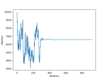
The algorithm correctly found the global minimum, x = 6590, and converged after about 300 iterations. Note that the function space as a whole is 10,000, so a brute-force approach would have taken 10,000 iterations. An animation showing the convergence of the solution to the global optimum as the temperature changes is also provided below:

Simulated annealing code: simulated_annealing.py